Quick Start Guide

Running the Simulation

In this guide we will set up a simple calculation, run the program, and interpret the results. This guide assumes that the python ThunderBoltz package has already been Installed.

For the first example, we will set up a Helium gas calculation, since the package already has a Helium model built-in. First, set up a file that will hold the python script to drive the simulation. In a new file run_example.py, write the following:

import os # Operating system interface for making directories

from thunderboltz import ThunderBoltz # Import the main simulation object
from thunderboltz.input import He_TB  # This is a built-in He model preset

# First we will make a folder in the current directory to house
# The simulation output / logging files.
os.makedirs("example_sim")

calc = ThunderBoltz(

     # Specify internal ThunderBoltz settings.
     DT=1e-10,             # Time step of 0.1 ns.
     NS=30000,             # Number of time steps.
     L=1e-6,               # The cell size (m).
     NP=[10000, 1000],     # 1e4 electrons, 1e3 Helium macroparticles.
     FV=[20000, 10000, 0], # Dump the electron velocities on steps 20000 and 30000.
     # ... etc.

     # Specify additional python interface settings in the same way.
     Ered=100,       # Fix the reduced field at 100 Townshend.
     eesd="uniform", # Use the uniform electron energy sharing ionization model.
     eadf="default", # Use isotropic elastic scattering.
     egen=False,     # Do not generate secondary electrons in ionization events.
     # ... etc.


     ### The package comes with a built-in Helium model that can be controlled
     ### with the following parameters.

     # This indicates use of the built in He model. It will automatically
     # set up the masses, charges, and cross sections for a fixed-background
     # Helium calculation.
     indeck=He_TB,
     # You may also specify up to what principle quantum number the
     # excitation cross sections will go.
     n=4,
     # Or how many points to sample the cross section model.
     nsamples=300,

     # Finally, specify a simulation directory where logging and output
     # files will be written.
     directory="example_sim",
)


# At this point, the ThunderBoltz object has been configured and is ready
# to run. To do this, just call the "run" method. This will write the
# necessary input files, compile the program from package source into the
# simulation directory, and execute the program in a subprocess.
calc.run(
    # By default, all output is written into files and not stdout,
    # but data can also be printed to stdout by setting
    std_banner=True,
)

# Once the calculation is finished, your python code will continue
# executing, and you can extract data from the ThunderBoltz object.

# This will extract step by step data for reaction counts/rates,
# electron mobility, drift velocity, and more.
ts = calc.get_timeseries()
# This will extract the same quantities but time averaged during the
# steady state period of the run.
steady_state = calc.get_ss_params()

# Sometimes it is easier to extract data once it is already been
# calculated. The next section will demonstrate how to asynchronously
# extract data after the calculation has finished in a new process.

This script can be run from the command line by simply executing

python run_example.py

Warning

When running and rerunning calculations, ensure that the specified simulation directory has no output files already present. ThunderBoltz will not overwrite these files when running more calculations. This will preserve your data, but prevent the python interface from being able to interpret the results.

For a full list available ThunderBoltz parameters, see Simulation Parameters.

Interpreting the Results

Some calculations of interest may take several hours, and so it is beneficial to run it once and explore the data later. It is easy to recover the output data from the output files after the calculation is finished like so:

# Import some python plotting tools
import matplotlib.pyplot as plt

# This will read single calculations and return ThunderBoltz objects.
from thunderboltz import read

# Ensure you are running this code from the same place as above, and
# just pass the location of the simulation directory.
calc = read("example_sim")

# Now all the same data will be available in the form of pandas DataFrames.
timeseries = calc.get_timeseries() # Returns timeseries data in a DataFrame.
steady_state = calc.get_ss_params() # Returns steady state data in a DataFrame.
velocity_data = calc.get_vdfs("all") # Returns all velocity dump data in a DataFrame.

# These frames are convenient because they can be easily manipulated and
# exported

# To export to csv:
timeseries.to_csv("example_sim/timeseries.csv", index=False)
steady_state.to_csv("example_sim/steady.csv", index=False)

# One can truncate the data row-wise. For example,
# the following will take data from last 20000 steps
# of the 30000 steps.
trunc = timeseries[timeseries.step >= 10000].copy()

# Or only look at certain columns

# This will extract the mean electron energy (MEe),
# the reduced electron mobility (mobN),
# and the Townshend ionization coefficient (a_n).
transport_params = timeseries[["MEe", "mobN", "a_n"]].copy()

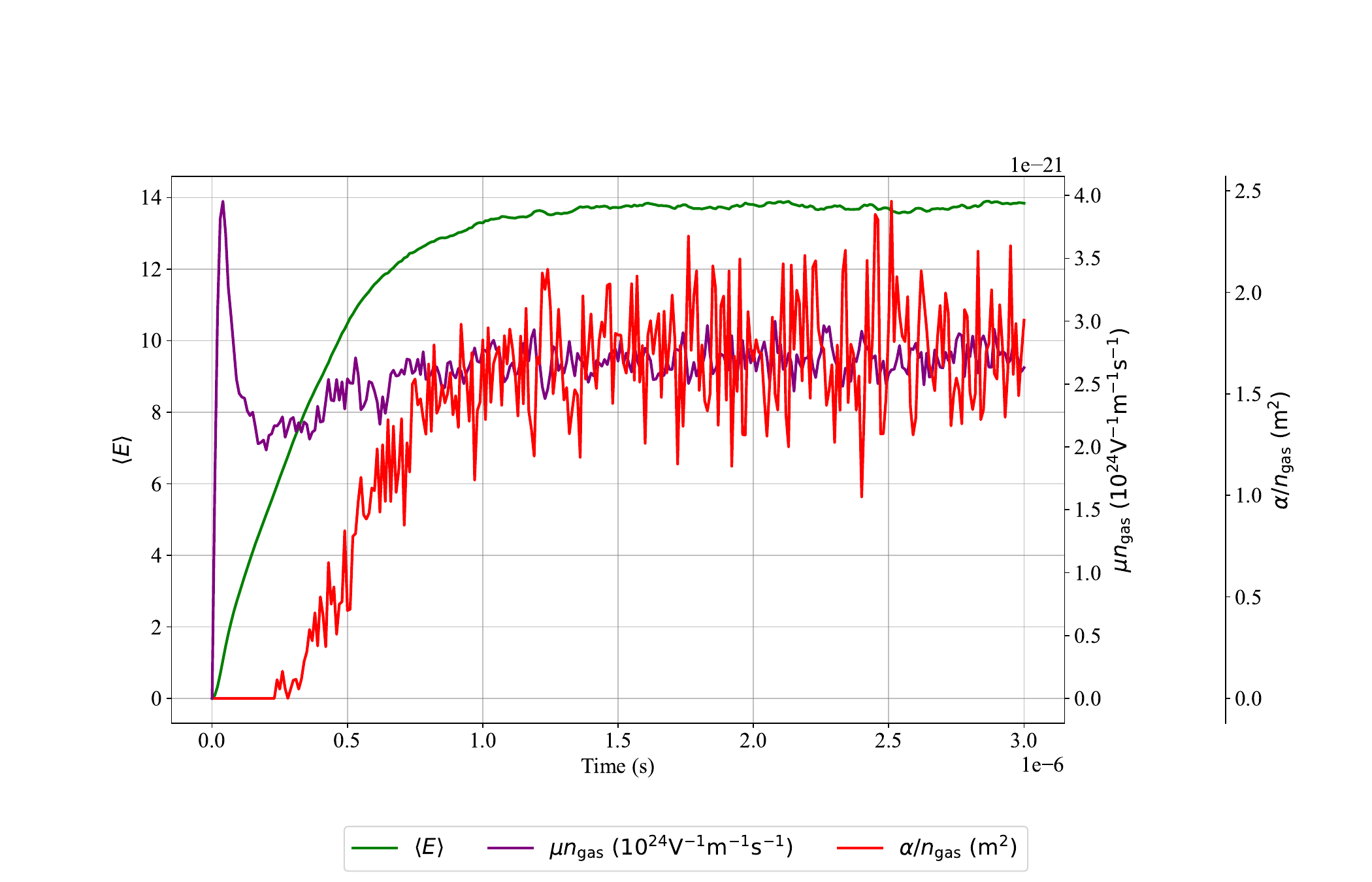
There are also some built-in plotting methods that can be accessed through the ThunderBoltz object.

# This will plot step by step data for any of the output
# parameters available in the time series table. Default
# is mean energy, mobility, and Townshend ionization coefficient
calc.plot_timeseries()

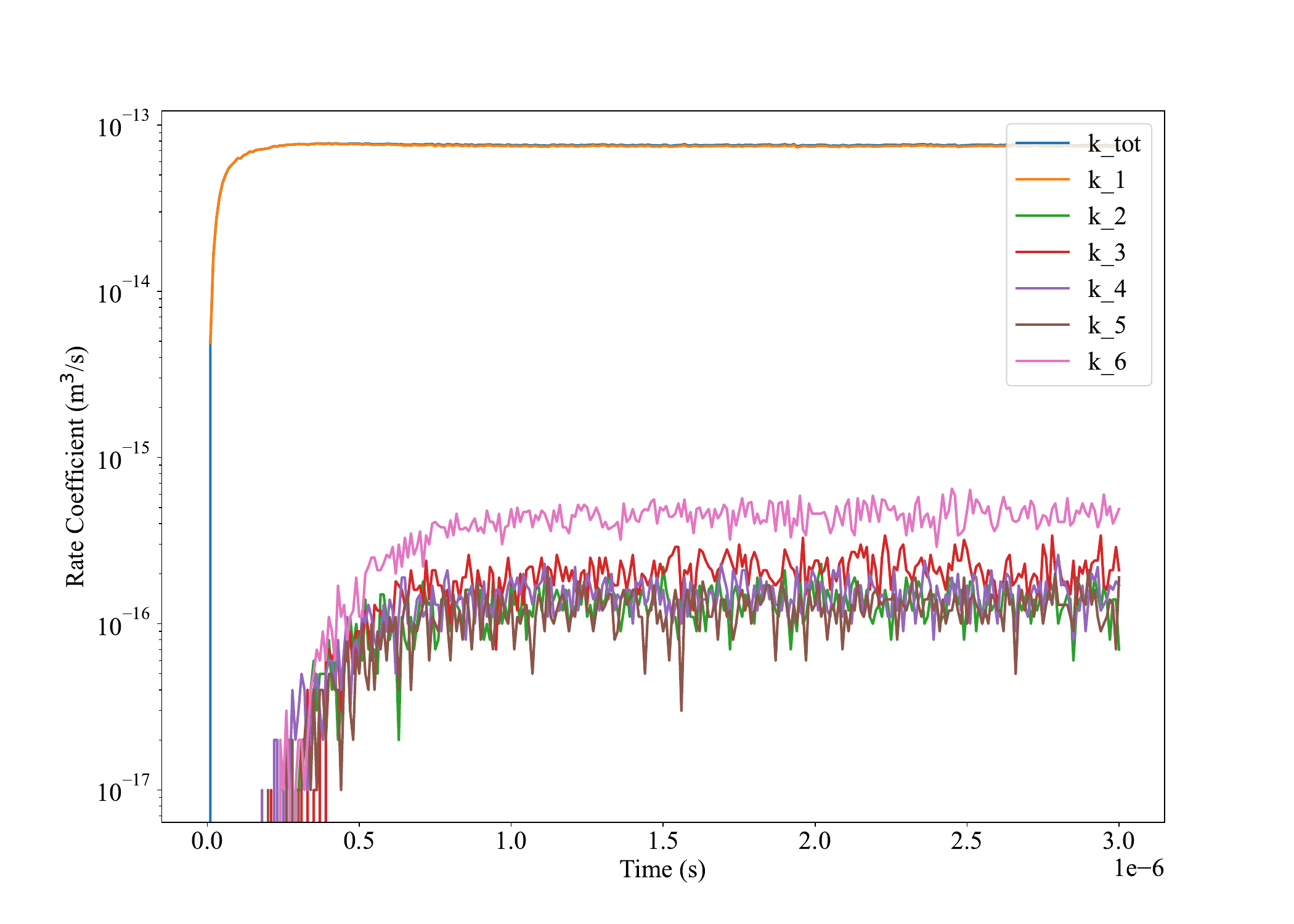
# This will plot the rate coefficients for every process.
calc.plot_rates()

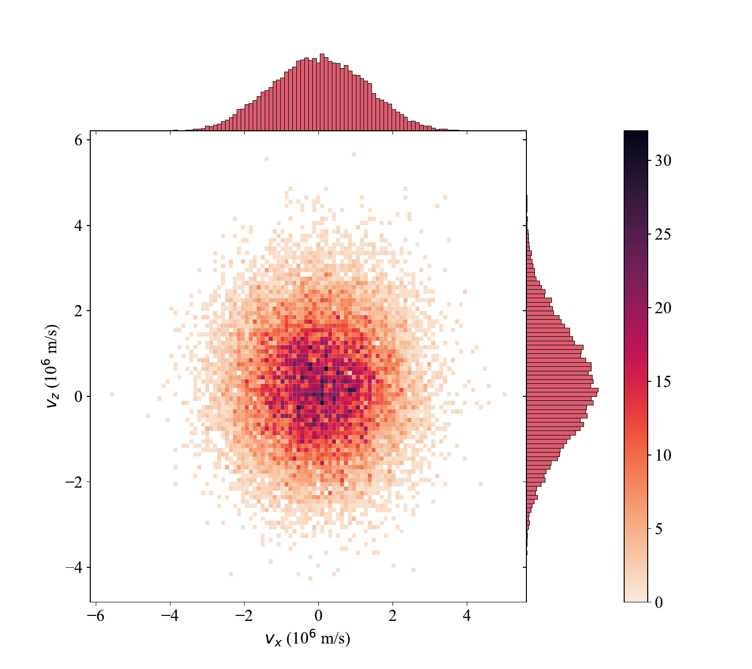
# This will plot a joint plot of the electron velocity distribution function
calc.plot_vdfs()

In order to actually view plots in a GUI, make sure to call the matplotlib function show,

# This will show a GUI and is required to actually display the plots.
plt.show()

For more details on the output parameter format, see Output Parameters.